The Bigger Picture

Introduction

Mistakes are probably the best way to improve at anything, so long as the proper care is taken in reflecting on them. My reflection often crosses the line into rumination, but is just as often perfectly healthy and helpful for growth. In this post, I will write about some mistakes I made on last year’s Advent of Code. These mistakes are mostly technical in nature, so for now my ruminations get to remain firmly in my own skull.

The first and most glaring error was approaching the problems when they became available, in the dead of night. There was no real reason to do it. It’s bad for sleep, bad for flow, and bad for arriving at correct conclusions. This was also a dreaded repeat mistake, having reared its head in the prior year’s competition. This time around, two time zones westward, I thought I would be able to stay sharp. As will become obvious, I did not succeed.

I am most interested in discussing a technical mistake - one that came up on Day 10 of the challenge. To be completely transparent, I want to discuss a particular mistake because I’m proud of its resolution - but that doesn’t mean that it’s not a major blunder. To cheer myself up, I will deliver the remainder of this piece using the oreo cookie approach, meaning I’ll start with what I did right.

Graph Theory is Overkill

I love graphs. I wrote an honors thesis on graph theory (maybe I’ll post it here?), so I will often go out of my way to solve a problem with graphs, even when a simpler, more elegant solution exists. For Day 10 of the 2023 Advent of Code, however, I resisted the temptation. The prompt is, as usual, a cutesy story about an adventurer trying to save Christmas. That day’s installment finds its intrepid protagonist staring down a pipe maze and an animal scurrying around a loop within it. The goal is to determine the length of the loop (half the length of the loop to be precise). The graph doesn’t need to be imagined, it’s very explicit. The vertex set is each section of pipe, and the edges are the connections between them. Here’s an example input to the problem:

7-F7-
.FJ|7
SJLL7
|F--J
LJ.LJ

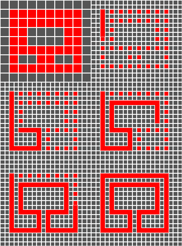
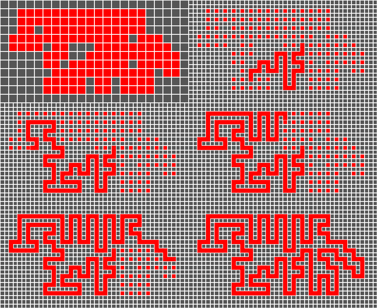
As I thought over the scenario to determine which graph representation to utilize, adjacency matrix or edge list (edge list would be much better), I realized that there is a much easier way. The starting point is given, so the entire loop can simply be stored in a list. The algorithm is simple - start at the ‘S’, and from its local neighborhood, determine which of its neighboring pipes is connected to it. Pick one arbitrarily, and from that pipe’s neighborhood, repeat the process, only instead of picking at random, move to the pipe that is novel. It’s guaranteed to be a loop, so eventually, it will terminate at the starting point. This approach requires very little preprocessing or memory overhead, and is very easily scalable. Here’s the (incomplete) python code for building the loop along with a visual representation of the algorithm operating on the sample input above:

lines = [x.strip() for x in f.readlines()]

    # starting coordinates
    s_y = [y for (l, y) in zip(lines, range(len(lines))) if 'S' in l][0]
    s_x = lines[s_y].index('S')

    old_cons = connecting(s_x, s_y, lines)
    new_cons = connecting(old_cons[0][0], old_cons[0][1], lines)

    loop = [(s_x, s_y), (old_cons[0][0], old_cons[0][1])]

    new_one = [p for p in new_cons if p not in [(s_x, s_y)]][0]

    while new_one not in loop:
        loop += [new_one]
        old_cons = new_cons
        new_cons = connecting(new_one[0], new_one[1], lines)
        new_one = [p for p in new_cons if p != loop[-2]][0]

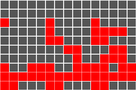
Once the loop is constructed, simply divide the length by two to arrive at our answer for the first phase of the puzzle. Done and dusted. Now, on to the tricky part.

An Overeager Application of Computational Geometry

Every AoC problem is split into two phases, and the second often includes a sharp increase in difficulty. The goal now is to take our original input and determine the area of the interior of the loop. I read this and my brain immediately jumped to a sweep algorithm. I first encountered this class of algorithms while passing the time in the tiny Frederick Douglass - Greater Rochester International Airport. Instead of thumbing through a paperback or binging Netflix, I had decided inexplicably to delve into the textbook Computational Geometry: Algorithms and Applications.

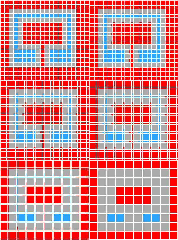
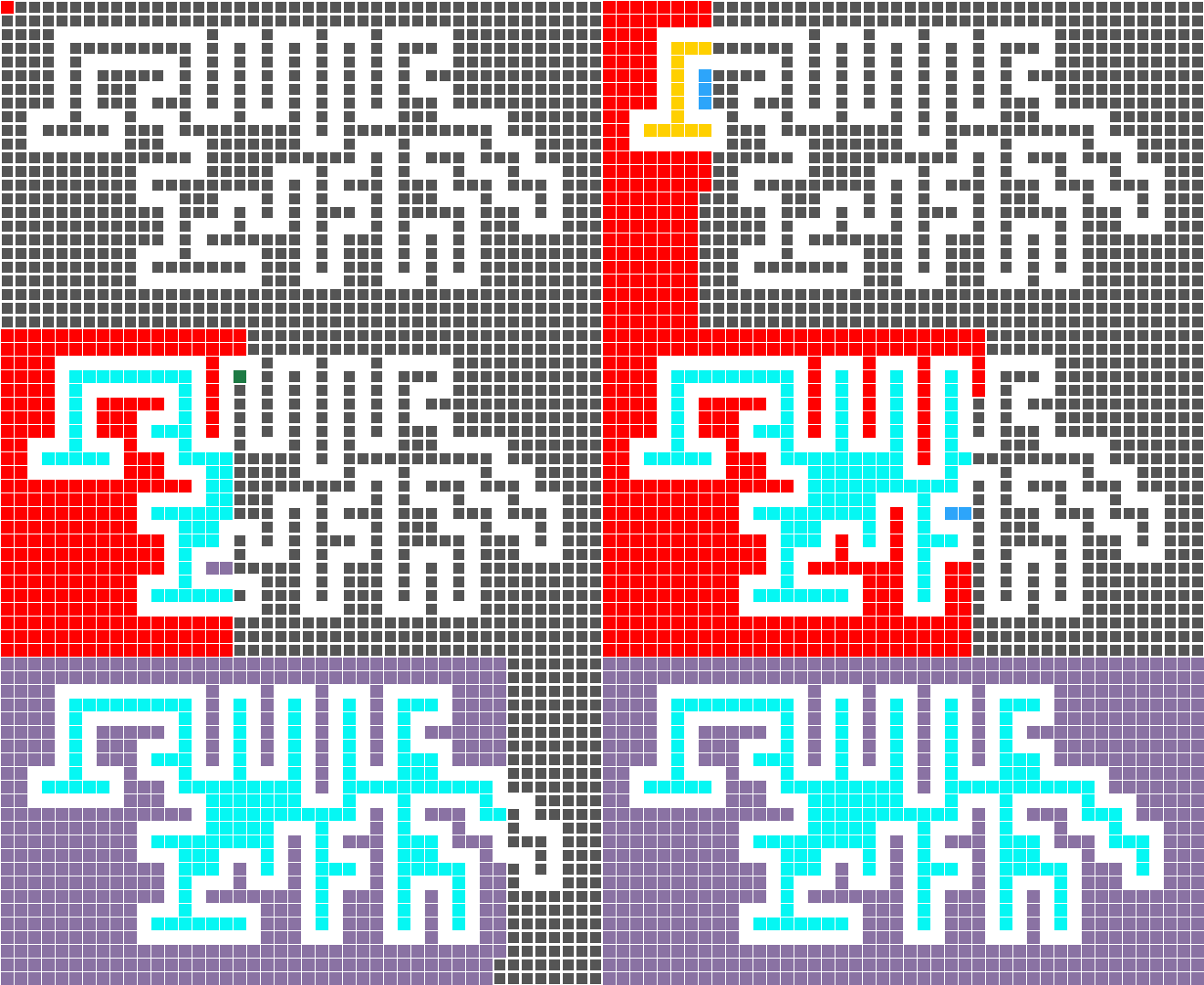
There is no better analogy for these algorithms than a document scanner. Essentially, imagine a line that sweeps across the plane, from left to right. The algorithm determines a property of the values on that line only using the values on one side of it. Then, the line sweeps to the next set of values, using the previous iteration’s discoveries to help determine the current batch. This is a geometric induction algorithm. Hastily, fueled in equal part by inspiration and sleep deprivation, I got coding. The particular property that my algorithm computes is a group membership, i.e. my algorithm partitions the input into connected sets of points. I decided to define the interior as the union of sets not connected to the edge. After I completed it, I threw together some edge cases in the problem domain to test, and they all passed. I will leave out the code, but include more visual aids in case my explanation of sweeping algorithms was lacking:

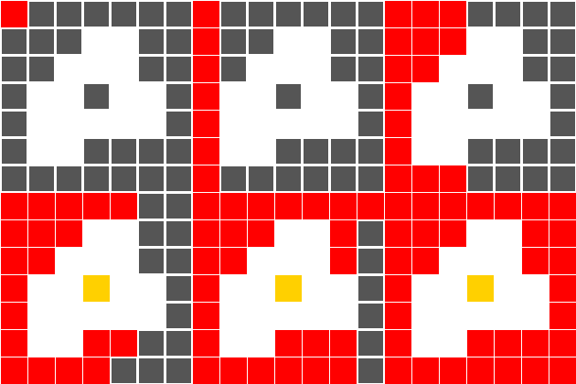
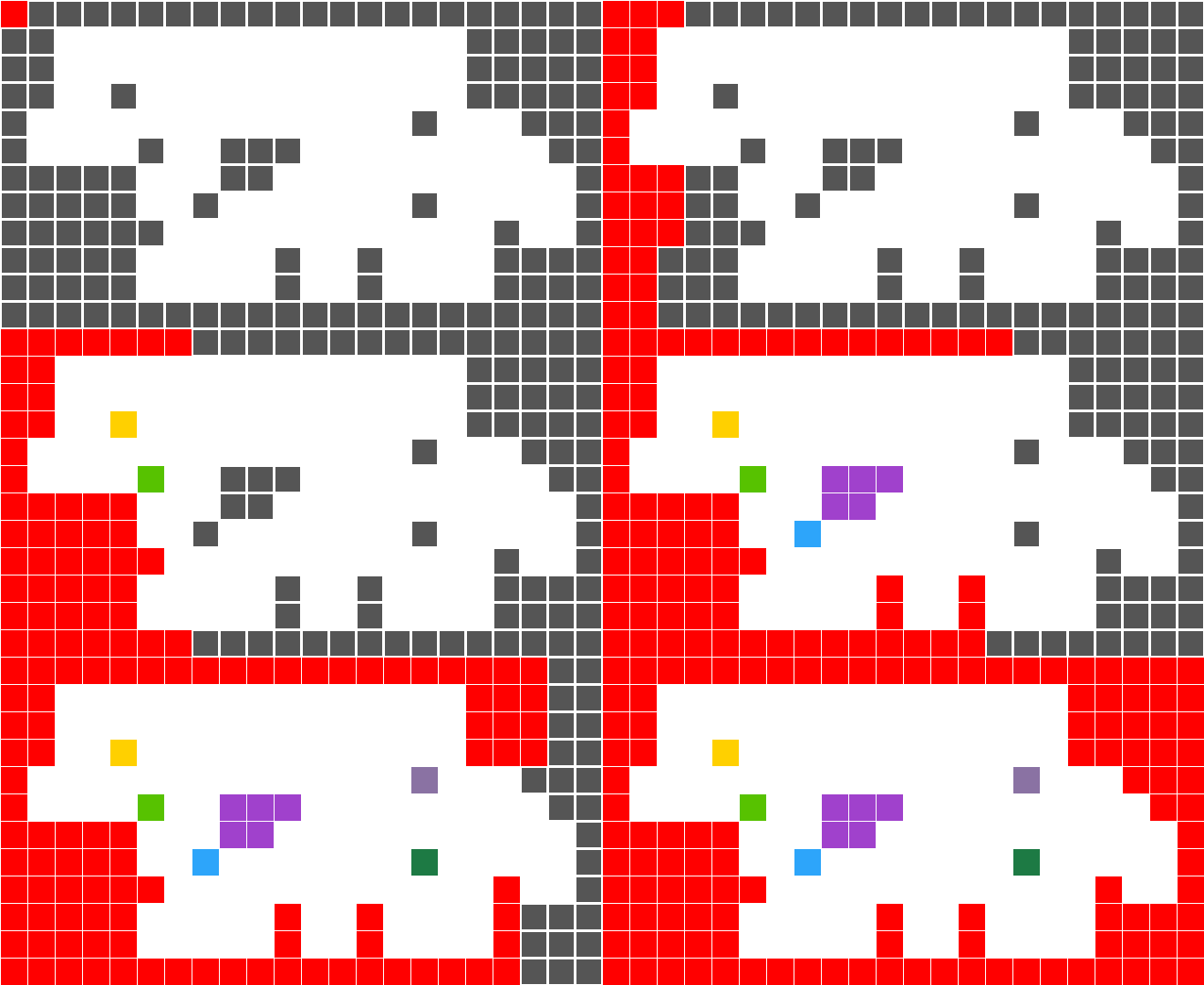
I’m satisfied, so I run my full puzzle input and viola! It’s wrong.

Disappointsments and Jordan Curves

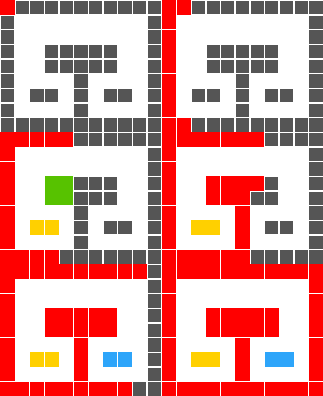
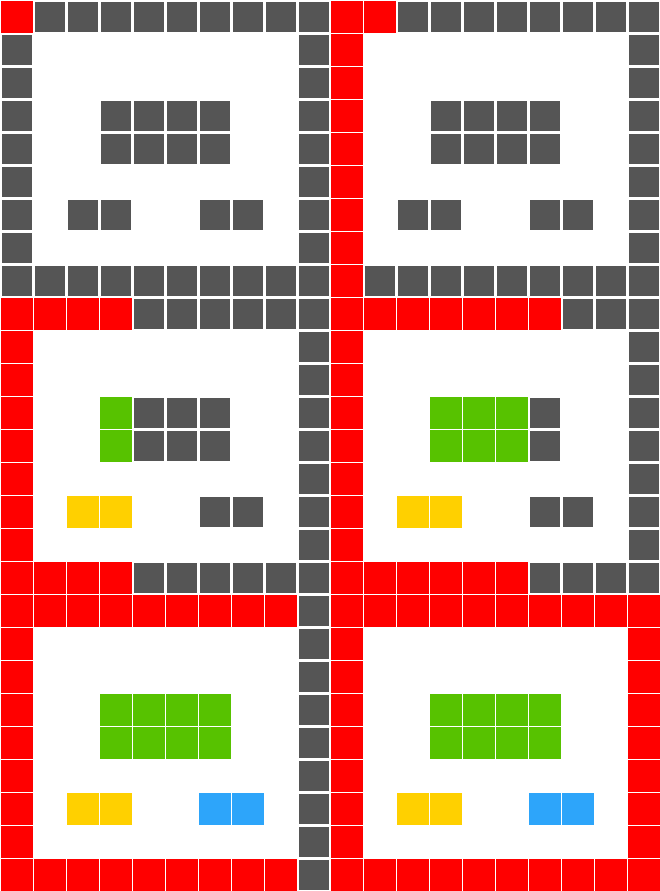
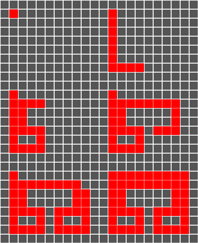
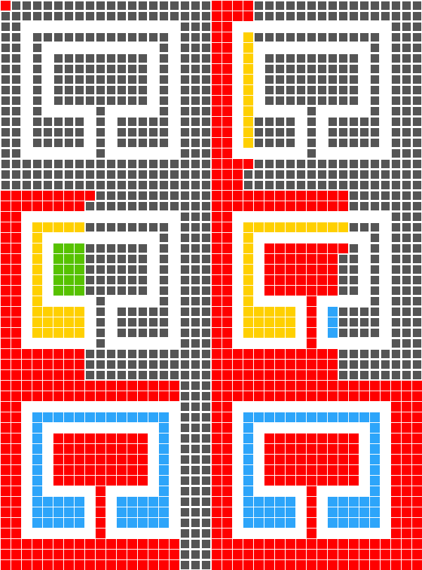
At first, I was perplexed as to why my solution was incorrect. For the above inputs, my algorithm outputs 1, 4, 12, and 10 respectively. These examples were taken directly from the prompt, so surely… wait. Those were the answers that I had expected, but they were not correct. Instead, the correct answers were 1, 4, 4, 8. I found where I had gone astray quite quickly - assumptions had done their dirty work. In my half asleep state, I had simply failed to fully read the prompt, and chose a definition directly counter to one given. I had decided that the interior was the set of squares that are not connected by a non-loop path to an edge square. The one picked by the author of the prompt - decidedly much more interesting and therefore better - was topological. They described the idea of “squeezing between pipes”, meaning there does not need to be a non-loop path to the edge for it to be considered part of the exterior. These are the inputs and the drawing process for the middle two examples from above:

...........
.S-------7.
.|F-----7|.
.||.....||.
.||.....||.
.|L-7.F-J|.
.|II|.|II|.
.L--J.L--J.
...........

..........
.S------7.
.|F----7|.
.||....||.
.||....||.
.|L-7F-J|.
.|..||..|.
.L--JL--J.
..........

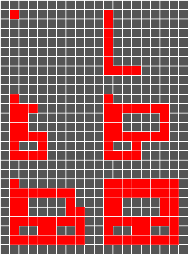
They are juxtaposed to demonstrate this concept. The group of eight central non-loop squares is part of the exterior in both cases. In the first one, it is obvious, and my algorithm detects this perfectly. In the second instance, they are part of the exterior because the path that connects them to the edge squeezes between the pipes.

I had to reconceptualize how I was thinking about the loop. It seemed that there was no way, in my current framing, to represent this idea of squeezing between pipes. I was disappointed, but decided that in order to solve the problem, I would need to seek a new framing - a new mathematical analogy. I found it in Jordan Curves.

A Jordan Curve is a closed, non-intersecting loop embedded in \(R^2\), the Euclidean Plane. One of the earliest theorems taught in introductory topology courses is the Jordan Curve Theorem, which states that every Jordan curve partitions \(R^2\) into exactly three sets - the loop itself, the interior, and the exterior. This interior is exactly the set that the original problem seems to be interested in. Since Jordan Curves are by definition embedded in \(R^2\) and non-intersecting, the squeezing between the pipes idea is realized by the fact that any two points along the curve, no matter how close they are, have points in between them. This is an extension of the completeness of real numbers to \(R^2\).

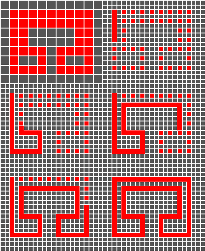
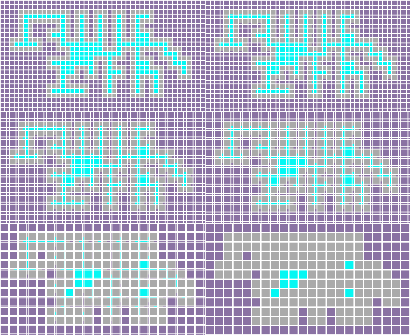
This is when a solution hit me - the algorithm I wrote would work! I just needed a change in perspective. The following is my attempt to explain, but the visual aid after it is worth all 400 words. The key realization is that my data structure is in fact not just a set of squares but a sequence of points. This loop can be thought of as embedded in \(Z^2\), and therefore could not rightly be thought of as a Jordan Curve. Those curves are non-overlapping, meaning between any two points on the curve that aren’t directly connected by a line of points entirely on the curve, there is a point on the line between them that isn’t on the curve. This run-on sentence is both dense and obvious once digested. It’s exactly what I explained in the previous paragraph, and it instantly disqualifies \(Z^2\) as a possible domain for a Jordan Curve. In the above examples, there are plenty of points on our curve that are abutting other points on the curve, but are not directly connected to them. Because this is a discrete space, there is no point between them, nothing that can help represent squeezing between.

In order to solve the problem, we need to extend the representation to allow for a point to be found on any two points on the curve. Note, this is different than just saying any two points. If we attempt to use a domain with all of the power of the real numbers, our sweeping algorithm must be adapted from a discrete algorithm to a continuous one, which is doable but unnecessary for the problem at hand. Instead, we adjoin to the existing domain points at each half value. The x-axis would now be the points \((0,0), (\frac{1}{2},0), (1,0), (\frac{3}{2},0)\) and so on. In this new domain, the loop, which only includes whole number points, is non-intersecting in the important way described above. The pipes can now be squeezed between. One final caveat is that after running the original algorithm on this new input, it’s important to only count the squares that are in the original domain. Fortunately, this is easily achieved by only considering whole number points.

For computational simplicity, this change in domain is equivalent to dilating from the origin by a scale factor of two, then filling in the blanks, i.e. adding to the loop the midpoints of each pair of sequential points of the loop. At the end, considering only whole number points is equivalent to considering only the points where both coordinates are even. See below code and visuals.

# zoom in (dilate by two) and fill in blanks
loop_zoomed = [(x * 2, y * 2) for (x, y) in loop]
for i in range(len(loop)):
    j = (i+1)%len(loop)
    avg = (loop[i][0] + loop[j][0], loop[i][1] + loop[j][1])
    loop_zoomed.insert(i*2+1, avg)

# ... consider only even points
if x % 2 == 0 and y % 2 == 0:
    total_enclosed += 1

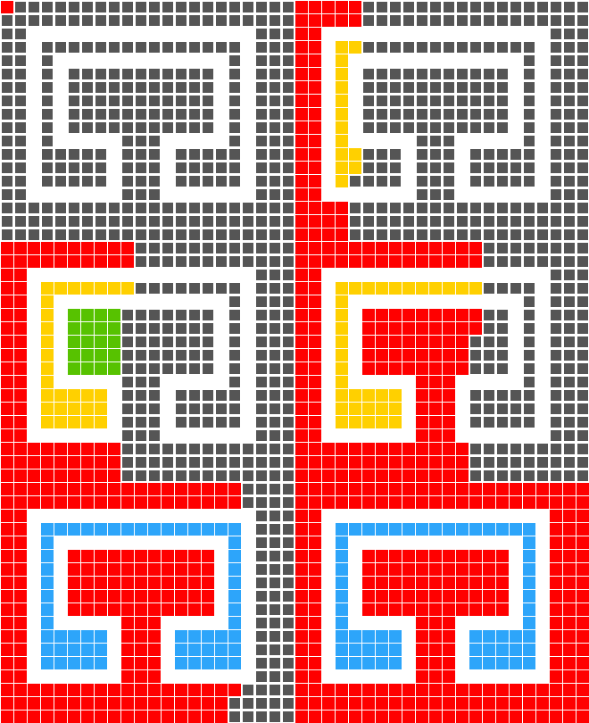
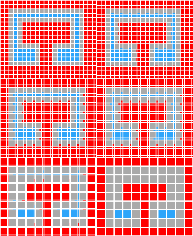
Drawing Conclusions

This new modified algorithm not only provides the correct solution for the sample, but also for the puzzle input. There were optimizations to be made, of course, but a correct solution was a correct solution. I am never glad to make an ass out of myself (as the old adage says), but I am pleased at the fact that I didn’t give up hope and start from scratch immediately. Having many tools in the toolbox, like prior knowledge of sweeping algorithms, leaves me both better equipped to solve problems and more likely to use the wrong tool. As I become more experienced, I realize that the specification of the problem domain is essential, but also that many problem domains are similar. I was able to approximate \(R^2\) - at least in terms of the properties that I required - by using \(Z^2\). It just required that I look at the bigger picture.

Finally, a bit of honesty. I’m always happy to wax poetic about the problem solving process, but my true motivation for this entire writeup is the visuals I’ve created. They are a pretty close approximation to what I saw when everything clicked. After that, I became much more focused on getting to the point that I could write the code that not only solves the problem but creates the visuals too. I used the Python library Pillow, and am quite pleased with the results. Because my main focus was the visuals, a mathy reader might find my justification for why extending the domain allows us to apply a sort of Jordan Curve theorem to be extremely hand wavy. That’s because it is. Perhaps someday I’ll put on my formal math pants and revisit that section, but for now, I’m hoping it at least provides some intuition.